import numpy as np
import scipy.stats as spst
import pandas as pd
import matplotlib.pyplot as plt
import seaborn as sns
import statsmodels.api as sm
import statsmodels.formula.api as smf
import duckdbSection 1 - Group 14
Abhishek Goyal (FT251004)
Anubhav Verma (FT251021)
Harshit Vashisht (FT251029)
N.V. Padmanayana (FT251048)
Waagmee Singh (FT251105)
Setup of database
We are going to use duckdb as our database engine. You can refer to the documentation here: Documentation. First, we will create a database called yelp.db in duckdb. We will persist this db on the harddrive because it might be too big to handle in your system RAM. That said, duckdb has in-RAM database capabilities as well. Of course, if you have a lot of RAM, you can use Pandas directly or use the in-RAM capabilities of duckdb. Once we execute the command below, we will have created the required db and connected to it as well. Once we have created the db, it will appear in the root folder of your project.
con = duckdb.connect("yelpdata.db")Now, we will import the csv files into four different tables namely restos, resto_reviews, users and user_friends. This is a onetime execution. You don’t need to execute the codecell below everytime you do the analysis. Once the tables are created, they will persist on the db in your root folder.
restos table comes from restuarants_train.csv (There is also a restuarants_test.csv. You do not need to worry about this test data now. This will be used to conduct a hackathon to predict star ratings later if we get time. ). The columns correspond to business.json in https://www.yelp.com/dataset/documentation/main
resto_reviews table comes from restaurant_reviews.csv. The columns correspond to review.json in https://www.yelp.com/dataset/documentation/main
users table comes from user.csv. The columns correspond to user.json in https://www.yelp.com/dataset/documentation/main
user_friends table comes from user_friends_full.csv. It was created by me. It shows the number of friends of each user in the social network of yelp.
con.sql("""
    CREATE TABLE restos AS
    FROM read_csv('yelp.restaurants_train.csv', sample_size = -1);
""")

con.sql("""
    CREATE TABLE resto_reviews AS
    FROM read_csv('yelp.restaurant_reviews.csv', sample_size = -1);
""")

con.sql("""
    CREATE TABLE users AS
    FROM read_csv('yelp.user.csv', sample_size = -1);
""")

con.sql("""
    CREATE TABLE user_friends AS
    FROM read_csv('yelp.user_friends_full.csv', sample_size = -1);
""")
Let us look at the first 5 rows of the restos table.
con.sql("""
    SELECT * FROM restos
    LIMIT 5;
""")
┌──────────────────────┬─────────────────────┬───────────┬───┬──────────────────────┬──────────────────────┐
│ name │ address │ city │ … │ attributes.Accepts… │ attributes.HairSpe… │
│ varchar │ varchar │ varchar │ │ boolean │ varchar │
├──────────────────────┼─────────────────────┼───────────┼───┼──────────────────────┼──────────────────────┤
│ Oskar Blues Taproom │ 921 Pearl St │ Boulder │ … │ NULL │ NULL │
│ Flying Elephants a… │ 7000 NE Airport Way │ Portland │ … │ NULL │ NULL │
│ Bob Likes Thai Food │ 3755 Main St │ Vancouver │ … │ NULL │ NULL │
│ Boxwood Biscuit │ 740 S High St │ Columbus │ … │ NULL │ NULL │
│ Mr G's Pizza & Subs │ 474 Lowell St │ Peabody │ … │ NULL │ NULL │
├──────────────────────┴─────────────────────┴───────────┴───┴──────────────────────┴──────────────────────┤
│ 5 rows 60 columns (5 shown) │
└──────────────────────────────────────────────────────────────────────────────────────────────────────────┘We can convert the results from duckdb into a pandas dataframe by appending .df() function as given below. This pandas dataframe can be used for further analysis in python.
df_restos = con.sql("""
    SELECT * FROM restos
    LIMIT 5;
""").df()
df_restos| name | address | city | state | postal_code | latitude | longitude | stars | review_count | is_open | ... | attributes.Smoking | attributes.DriveThru | attributes.BYOBCorkage | attributes.Corkage | attributes.RestaurantsCounterService | attributes.DietaryRestrictions | attributes.AgesAllowed | attributes.Open24Hours | attributes.AcceptsInsurance | attributes.HairSpecializesIn | |
|---|---|---|---|---|---|---|---|---|---|---|---|---|---|---|---|---|---|---|---|---|---|
| 0 | Oskar Blues Taproom | 921 Pearl St | Boulder | CO | 80302 | 40.017544 | -105.283348 | 4.0 | 86 | 1 | ... | None | None | None | None | NaN | None | None | NaN | NaN | None |
| 1 | Flying Elephants at PDX | 7000 NE Airport Way | Portland | OR | 97218 | 45.588906 | -122.593331 | 4.0 | 126 | 1 | ... | None | None | None | None | NaN | None | None | NaN | NaN | None |
| 2 | Bob Likes Thai Food | 3755 Main St | Vancouver | BC | V5V | 49.251342 | -123.101333 | 3.5 | 169 | 1 | ... | None | None | None | None | NaN | None | None | NaN | NaN | None |
| 3 | Boxwood Biscuit | 740 S High St | Columbus | OH | 43206 | 39.947007 | -82.997471 | 4.5 | 11 | 1 | ... | None | None | None | None | NaN | None | None | NaN | NaN | None |
| 4 | Mr G's Pizza & Subs | 474 Lowell St | Peabody | MA | 01960 | 42.541155 | -70.973438 | 4.0 | 39 | 1 | ... | None | None | None | None | NaN | None | None | NaN | NaN | None |
5 rows × 60 columns
Let us look at the columns in each of the tables.
con.sql("""
    DESCRIBE restos
""").df()| column_name | column_type | null | key | default | extra | |
|---|---|---|---|---|---|---|
| 0 | name | VARCHAR | YES | None | None | None |
| 1 | address | VARCHAR | YES | None | None | None |
| 2 | city | VARCHAR | YES | None | None | None |
| 3 | state | VARCHAR | YES | None | None | None |
| 4 | postal_code | VARCHAR | YES | None | None | None |
| 5 | latitude | DOUBLE | YES | None | None | None |
| 6 | longitude | DOUBLE | YES | None | None | None |
| 7 | stars | DOUBLE | YES | None | None | None |
| 8 | review_count | BIGINT | YES | None | None | None |
| 9 | is_open | BIGINT | YES | None | None | None |
| 10 | attributes.RestaurantsTableService | VARCHAR | YES | None | None | None |
| 11 | attributes.WiFi | VARCHAR | YES | None | None | None |
| 12 | attributes.BikeParking | VARCHAR | YES | None | None | None |
| 13 | attributes.BusinessParking | VARCHAR | YES | None | None | None |
| 14 | attributes.BusinessAcceptsCreditCards | VARCHAR | YES | None | None | None |
| 15 | attributes.RestaurantsReservations | VARCHAR | YES | None | None | None |
| 16 | attributes.WheelchairAccessible | VARCHAR | YES | None | None | None |
| 17 | attributes.Caters | VARCHAR | YES | None | None | None |
| 18 | attributes.OutdoorSeating | VARCHAR | YES | None | None | None |
| 19 | attributes.RestaurantsGoodForGroups | VARCHAR | YES | None | None | None |
| 20 | attributes.HappyHour | VARCHAR | YES | None | None | None |
| 21 | attributes.BusinessAcceptsBitcoin | BOOLEAN | YES | None | None | None |
| 22 | attributes.RestaurantsPriceRange2 | VARCHAR | YES | None | None | None |
| 23 | attributes.Ambience | VARCHAR | YES | None | None | None |
| 24 | attributes.HasTV | VARCHAR | YES | None | None | None |
| 25 | attributes.Alcohol | VARCHAR | YES | None | None | None |
| 26 | attributes.GoodForMeal | VARCHAR | YES | None | None | None |
| 27 | attributes.DogsAllowed | VARCHAR | YES | None | None | None |
| 28 | attributes.RestaurantsTakeOut | VARCHAR | YES | None | None | None |
| 29 | attributes.NoiseLevel | VARCHAR | YES | None | None | None |
| 30 | attributes.RestaurantsAttire | VARCHAR | YES | None | None | None |
| 31 | attributes.RestaurantsDelivery | VARCHAR | YES | None | None | None |
| 32 | categories | VARCHAR | YES | None | None | None |
| 33 | hours.Monday | VARCHAR | YES | None | None | None |
| 34 | hours.Tuesday | VARCHAR | YES | None | None | None |
| 35 | hours.Wednesday | VARCHAR | YES | None | None | None |
| 36 | hours.Thursday | VARCHAR | YES | None | None | None |
| 37 | hours.Friday | VARCHAR | YES | None | None | None |
| 38 | hours.Saturday | VARCHAR | YES | None | None | None |
| 39 | hours.Sunday | VARCHAR | YES | None | None | None |
| 40 | int_business_id | BIGINT | YES | None | None | None |
| 41 | attributes.GoodForKids | VARCHAR | YES | None | None | None |
| 42 | attributes.ByAppointmentOnly | BOOLEAN | YES | None | None | None |
| 43 | attributes | VARCHAR | YES | None | None | None |
| 44 | hours | VARCHAR | YES | None | None | None |
| 45 | attributes.Music | VARCHAR | YES | None | None | None |
| 46 | attributes.GoodForDancing | VARCHAR | YES | None | None | None |
| 47 | attributes.BestNights | VARCHAR | YES | None | None | None |
| 48 | attributes.BYOB | VARCHAR | YES | None | None | None |
| 49 | attributes.CoatCheck | VARCHAR | YES | None | None | None |
| 50 | attributes.Smoking | VARCHAR | YES | None | None | None |
| 51 | attributes.DriveThru | VARCHAR | YES | None | None | None |
| 52 | attributes.BYOBCorkage | VARCHAR | YES | None | None | None |
| 53 | attributes.Corkage | VARCHAR | YES | None | None | None |
| 54 | attributes.RestaurantsCounterService | BOOLEAN | YES | None | None | None |
| 55 | attributes.DietaryRestrictions | VARCHAR | YES | None | None | None |
| 56 | attributes.AgesAllowed | VARCHAR | YES | None | None | None |
| 57 | attributes.Open24Hours | BOOLEAN | YES | None | None | None |
| 58 | attributes.AcceptsInsurance | BOOLEAN | YES | None | None | None |
| 59 | attributes.HairSpecializesIn | VARCHAR | YES | None | None | None |
con.sql("""
    DESCRIBE resto_reviews
""")
┌────────────────────┬─────────────┬─────────┬─────────┬─────────┬─────────┐
│ column_name │ column_type │ null │ key │ default │ extra │
│ varchar │ varchar │ varchar │ varchar │ varchar │ varchar │
├────────────────────┼─────────────┼─────────┼─────────┼─────────┼─────────┤
│ stars │ BIGINT │ YES │ NULL │ NULL │ NULL │
│ useful │ BIGINT │ YES │ NULL │ NULL │ NULL │
│ funny │ BIGINT │ YES │ NULL │ NULL │ NULL │
│ cool │ BIGINT │ YES │ NULL │ NULL │ NULL │
│ text │ VARCHAR │ YES │ NULL │ NULL │ NULL │
│ date │ TIMESTAMP │ YES │ NULL │ NULL │ NULL │
│ int_business_id │ BIGINT │ YES │ NULL │ NULL │ NULL │
│ int_user_id │ BIGINT │ YES │ NULL │ NULL │ NULL │
│ int_rest_review_id │ BIGINT │ YES │ NULL │ NULL │ NULL │
└────────────────────┴─────────────┴─────────┴─────────┴─────────┴─────────┘con.sql("""
DESCRIBE users
""")┌────────────────────┬─────────────┬─────────┬─────────┬─────────┬─────────┐
│ column_name │ column_type │ null │ key │ default │ extra │
│ varchar │ varchar │ varchar │ varchar │ varchar │ varchar │
├────────────────────┼─────────────┼─────────┼─────────┼─────────┼─────────┤
│ review_count │ BIGINT │ YES │ NULL │ NULL │ NULL │
│ yelping_since │ TIMESTAMP │ YES │ NULL │ NULL │ NULL │
│ useful │ BIGINT │ YES │ NULL │ NULL │ NULL │
│ funny │ BIGINT │ YES │ NULL │ NULL │ NULL │
│ cool │ BIGINT │ YES │ NULL │ NULL │ NULL │
│ elite │ VARCHAR │ YES │ NULL │ NULL │ NULL │
│ fans │ BIGINT │ YES │ NULL │ NULL │ NULL │
│ average_stars │ DOUBLE │ YES │ NULL │ NULL │ NULL │
│ compliment_hot │ BIGINT │ YES │ NULL │ NULL │ NULL │
│ compliment_more │ BIGINT │ YES │ NULL │ NULL │ NULL │
│ compliment_profile │ BIGINT │ YES │ NULL │ NULL │ NULL │
│ compliment_cute │ BIGINT │ YES │ NULL │ NULL │ NULL │
│ compliment_list │ BIGINT │ YES │ NULL │ NULL │ NULL │
│ compliment_note │ BIGINT │ YES │ NULL │ NULL │ NULL │
│ compliment_plain │ BIGINT │ YES │ NULL │ NULL │ NULL │
│ compliment_cool │ BIGINT │ YES │ NULL │ NULL │ NULL │
│ compliment_funny │ BIGINT │ YES │ NULL │ NULL │ NULL │
│ compliment_writer │ BIGINT │ YES │ NULL │ NULL │ NULL │
│ compliment_photos │ BIGINT │ YES │ NULL │ NULL │ NULL │
│ int_user_id │ BIGINT │ YES │ NULL │ NULL │ NULL │
├────────────────────┴─────────────┴─────────┴─────────┴─────────┴─────────┤
│ 20 rows 6 columns │
└──────────────────────────────────────────────────────────────────────────┘con.sql("""
DESCRIBE user_friends
""")┌─────────────┬─────────────┬─────────┬─────────┬─────────┬─────────┐
│ column_name │ column_type │ null │ key │ default │ extra │
│ varchar │ varchar │ varchar │ varchar │ varchar │ varchar │
├─────────────┼─────────────┼─────────┼─────────┼─────────┼─────────┤
│ int_user_id │ BIGINT │ YES │ NULL │ NULL │ NULL │
│ num_friends │ BIGINT │ YES │ NULL │ NULL │ NULL │
└─────────────┴─────────────┴─────────┴─────────┴─────────┴─────────┘Descriptive analysis
Average stars received by restaurants.
con.sql("""
    SELECT avg(stars) FROM restos
""")
┌───────────────────┐
│ avg(stars) │
│ double │
├───────────────────┤
│ 3.527858606557377 │
└───────────────────┘We will select the stars column from restos and plot a histogram of stars.
df_temp = con.sql("""
    SELECT stars FROM restos
""").df()
df_temp| stars | |
|---|---|
| 0 | 4.0 |
| 1 | 4.0 |
| 2 | 3.5 |
| 3 | 4.5 |
| 4 | 4.0 |
| ... | ... |
| 48795 | 2.0 |
| 48796 | 3.0 |
| 48797 | 3.0 |
| 48798 | 4.0 |
| 48799 | 4.5 |
48800 rows × 1 columns
sns.displot(data = df_temp, x = "stars", kind = "hist", color = "Green")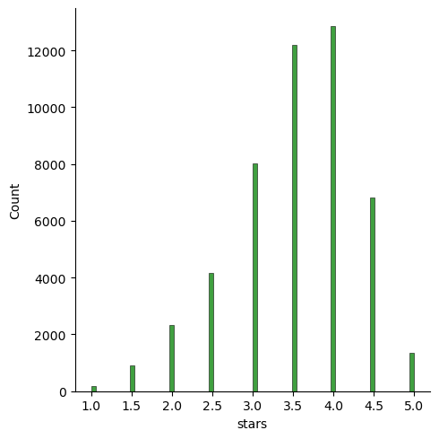
Average stars on yelp received by restaurants grouped by state.
df_temp = con.sql("""
    SELECT state, avg(stars) as avg_stars FROM restos
    GROUP BY state
    ORDER BY avg_stars DESC
""").df()
df_temp| state | avg_stars | |
|---|---|---|
| 0 | ABE | 4.500000 |
| 1 | NH | 4.000000 |
| 2 | OR | 3.752074 |
| 3 | TX | 3.656262 |
| 4 | CO | 3.587216 |
| 5 | FL | 3.521030 |
| 6 | MN | 3.500000 |
| 7 | MA | 3.480819 |
| 8 | BC | 3.454463 |
| 9 | WA | 3.450202 |
| 10 | OH | 3.421853 |
| 11 | GA | 3.399796 |
| 12 | KY | 2.000000 |
| 13 | VA | 2.000000 |
| 14 | KS | 2.000000 |
| 15 | WY | 1.500000 |
Let us look at how many restaurants provide WiFi.
con.sql("""
    SELECT DISTINCT "attributes.WiFi" FROM restos
""").df()| attributes.WiFi | |
|---|---|
| 0 | u'no' |
| 1 | u'paid' |
| 2 | 'paid' |
| 3 | u'free' |
| 4 | None |
| 5 | 'free' |
| 6 | 'no' |
| 7 | None |
df_temp = con.sql("""
    SELECT "attributes.WiFi" AS wifi, count("attributes.WiFi") AS count FROM restos
    GROUP BY wifi
""").df()
df_temp| wifi | count | |
|---|---|---|
| 0 | 'free' | 5496 |
| 1 | u'paid' | 184 |
| 2 | u'free' | 14994 |
| 3 | None | 29 |
| 4 | u'no' | 11706 |
| 5 | 'no' | 4394 |
| 6 | 'paid' | 81 |
| 7 | None | 0 |
Of course we will need to correct the data because, as you can see, the values of the variable are not clean. There seems to be repetitions of the same thing mentioned in two different ways.
df_new = pd.DataFrame({
    "wifi": [
        "None",
        "Free",
        "No",
        "Paid"
    ],
    "count": [
        (df_temp["count"][0] + df_temp["count"][7]),
        (df_temp["count"][1] + df_temp["count"][3]),
        (df_temp["count"][2] + df_temp["count"][5]),
        (df_temp["count"][4] + df_temp["count"][6])
    ]
})
df_new| wifi | count | |
|---|---|---|
| 0 | None | 5496 |
| 1 | Free | 213 |
| 2 | No | 19388 |
| 3 | Paid | 11787 |
Let us find aggregates of useful votes recevied by reviews grouped by star ratings.
df_temp = con.sql("""
    SELECT stars, sum(useful) as sum_useful, avg(useful) as avg_useful, max(useful) AS max_useful FROM resto_reviews
    GROUP BY stars
    ORDER BY stars ASC
""").df()
df_temp| stars | sum_useful | avg_useful | max_useful | |
|---|---|---|---|---|
| 0 | 1 | 239163.0 | 1.256445 | 146 |
| 1 | 2 | 184718.0 | 1.192214 | 260 |
| 2 | 3 | 216230.0 | 1.000694 | 177 |
| 3 | 4 | 454666.0 | 1.036895 | 411 |
| 4 | 5 | 556257.0 | 0.825011 | 223 |
sns.catplot(
    data=df_temp,
    x="stars",
    y="sum_useful",
    kind="bar",
    palette='magma',
    height=6,
    aspect=1.5,
    edgecolor="black"
)
C:\Users\A\AppData\Local\Temp\ipykernel_15224\656945628.py:1: FutureWarning:
Passing `palette` without assigning `hue` is deprecated and will be removed in v0.14.0. Assign the `x` variable to `hue` and set `legend=False` for the same effect.
sns.catplot(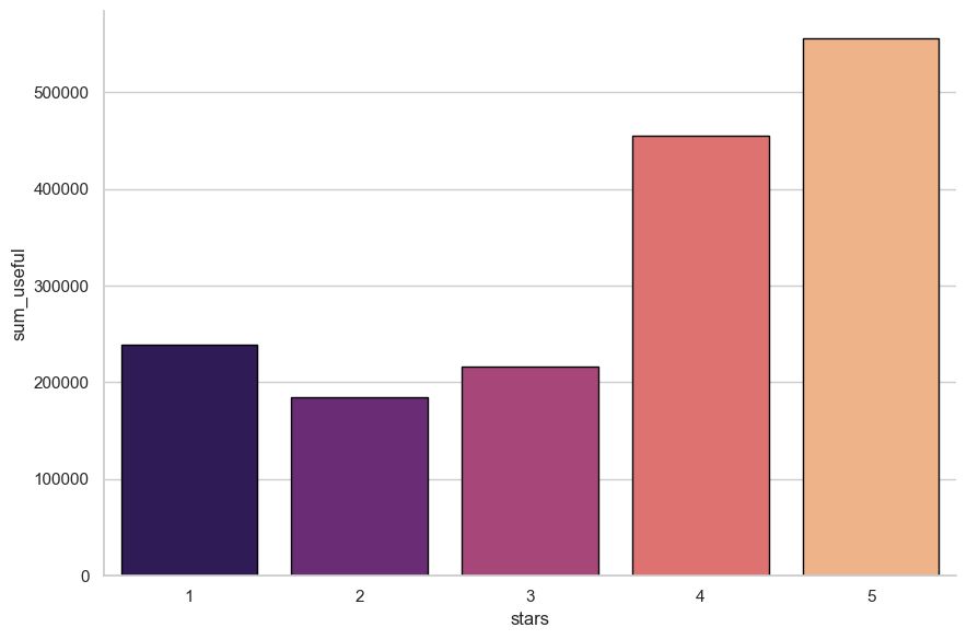
Part 1 - Exploratory Data Analysis
Data cleaning and merging
df_restos = con.sql('select * from restos').df()
df_resto_reviews = con.sql('select * from resto_reviews').df()
df_users = con.sql('select * from users').df()
df_user_friends = con.sql('select * from user_friends').df()
The tables for each of the CSV files look as below
df_restos.head(5)| name | address | city | state | postal_code | latitude | longitude | stars | review_count | is_open | ... | attributes.Smoking | attributes.DriveThru | attributes.BYOBCorkage | attributes.Corkage | attributes.RestaurantsCounterService | attributes.DietaryRestrictions | attributes.AgesAllowed | attributes.Open24Hours | attributes.AcceptsInsurance | attributes.HairSpecializesIn | |
|---|---|---|---|---|---|---|---|---|---|---|---|---|---|---|---|---|---|---|---|---|---|
| 0 | Oskar Blues Taproom | 921 Pearl St | Boulder | CO | 80302 | 40.017544 | -105.283348 | 4.0 | 86 | 1 | ... | None | None | None | None | NaN | None | None | NaN | NaN | None |
| 1 | Flying Elephants at PDX | 7000 NE Airport Way | Portland | OR | 97218 | 45.588906 | -122.593331 | 4.0 | 126 | 1 | ... | None | None | None | None | NaN | None | None | NaN | NaN | None |
| 2 | Bob Likes Thai Food | 3755 Main St | Vancouver | BC | V5V | 49.251342 | -123.101333 | 3.5 | 169 | 1 | ... | None | None | None | None | NaN | None | None | NaN | NaN | None |
| 3 | Boxwood Biscuit | 740 S High St | Columbus | OH | 43206 | 39.947007 | -82.997471 | 4.5 | 11 | 1 | ... | None | None | None | None | NaN | None | None | NaN | NaN | None |
| 4 | Mr G's Pizza & Subs | 474 Lowell St | Peabody | MA | 01960 | 42.541155 | -70.973438 | 4.0 | 39 | 1 | ... | None | None | None | None | NaN | None | None | NaN | NaN | None |
5 rows × 60 columns
df_resto_reviews.head(5)| stars | useful | funny | cool | text | date | int_business_id | int_user_id | int_rest_review_id | |
|---|---|---|---|---|---|---|---|---|---|
| 0 | 2 | 1 | 1 | 1 | I've stayed at many Marriott and Renaissance M... | 2010-01-08 02:29:15 | 4954 | 6319642 | 2 |
| 1 | 2 | 0 | 0 | 0 | The setting is perfectly adequate, and the foo... | 2006-04-16 02:58:44 | 14180 | 292901 | 5 |
| 2 | 5 | 0 | 0 | 0 | I work in the Pru and this is the most afforda... | 2014-05-07 18:10:21 | 11779 | 6336225 | 7 |
| 3 | 5 | 5 | 3 | 3 | I loved everything about this place. I've only... | 2014-02-05 21:09:05 | 3216 | 552519 | 12 |
| 4 | 4 | 0 | 0 | 0 | I think their rice dishes are way better than ... | 2017-05-26 03:05:46 | 8748 | 544027 | 16 |
df_users.head(5)| review_count | yelping_since | useful | funny | cool | elite | fans | average_stars | compliment_hot | compliment_more | compliment_profile | compliment_cute | compliment_list | compliment_note | compliment_plain | compliment_cool | compliment_funny | compliment_writer | compliment_photos | int_user_id | |
|---|---|---|---|---|---|---|---|---|---|---|---|---|---|---|---|---|---|---|---|---|
| 0 | 1220 | 2005-03-14 20:26:35 | 15038 | 10030 | 11291 | 2006,2007,2008,2009,2010,2011,2012,2013,2014 | 1357 | 3.85 | 1710 | 163 | 190 | 361 | 147 | 1212 | 5691 | 2541 | 2541 | 815 | 323 | 1 |
| 1 | 2136 | 2007-08-10 19:01:51 | 21272 | 10289 | 18046 | 2007,2008,2009,2010,2011,2012,2013,2014,2015,2... | 1025 | 4.09 | 1632 | 87 | 94 | 232 | 96 | 1187 | 3293 | 2205 | 2205 | 472 | 294 | 1248 |
| 2 | 119 | 2007-02-07 15:47:53 | 188 | 128 | 130 | 2010,2011 | 16 | 3.76 | 22 | 1 | 3 | 0 | 0 | 5 | 20 | 31 | 31 | 3 | 1 | 11604 |
| 3 | 987 | 2009-02-09 16:14:29 | 7234 | 4722 | 4035 | 2009,2010,2011,2012,2013,2014 | 420 | 3.77 | 1180 | 129 | 93 | 219 | 90 | 1120 | 4510 | 1566 | 1566 | 391 | 326 | 2278 |
| 4 | 495 | 2008-03-03 04:57:05 | 1577 | 727 | 1124 | 2009,2010,2011 | 47 | 3.72 | 248 | 19 | 32 | 16 | 15 | 77 | 131 | 310 | 310 | 98 | 44 | 13481 |
df_user_friends.head(5)| int_user_id | num_friends | |
|---|---|---|
| 0 | 1 | 5813 |
| 1 | 1248 | 6296 |
| 2 | 11604 | 835 |
| 3 | 2278 | 1452 |
| 4 | 13481 | 532 |
df_restos.info()<class 'pandas.core.frame.DataFrame'>
RangeIndex: 48800 entries, 0 to 48799
Data columns (total 60 columns):
# Column Non-Null Count Dtype
--- ------ -------------- -----
0 name 48800 non-null object
1 address 48378 non-null object
2 city 48800 non-null object
3 state 48800 non-null object
4 postal_code 48776 non-null object
5 latitude 48800 non-null float64
6 longitude 48800 non-null float64
7 stars 48800 non-null float64
8 review_count 48800 non-null int64
9 is_open 48800 non-null int64
10 attributes.RestaurantsTableService 18523 non-null object
11 attributes.WiFi 36884 non-null object
12 attributes.BikeParking 33715 non-null object
13 attributes.BusinessParking 44235 non-null object
14 attributes.BusinessAcceptsCreditCards 39552 non-null object
15 attributes.RestaurantsReservations 42037 non-null object
16 attributes.WheelchairAccessible 12628 non-null object
17 attributes.Caters 33288 non-null object
18 attributes.OutdoorSeating 42636 non-null object
19 attributes.RestaurantsGoodForGroups 40952 non-null object
20 attributes.HappyHour 12774 non-null object
21 attributes.BusinessAcceptsBitcoin 5952 non-null object
22 attributes.RestaurantsPriceRange2 43154 non-null object
23 attributes.Ambience 39676 non-null object
24 attributes.HasTV 39971 non-null object
25 attributes.Alcohol 39435 non-null object
26 attributes.GoodForMeal 27935 non-null object
27 attributes.DogsAllowed 11071 non-null object
28 attributes.RestaurantsTakeOut 45727 non-null object
29 attributes.NoiseLevel 34457 non-null object
30 attributes.RestaurantsAttire 38941 non-null object
31 attributes.RestaurantsDelivery 44650 non-null object
32 categories 48800 non-null object
33 hours.Monday 36880 non-null object
34 hours.Tuesday 38586 non-null object
35 hours.Wednesday 40018 non-null object
36 hours.Thursday 40597 non-null object
37 hours.Friday 40775 non-null object
38 hours.Saturday 39370 non-null object
39 hours.Sunday 34455 non-null object
40 int_business_id 48800 non-null int64
41 attributes.GoodForKids 40477 non-null object
42 attributes.ByAppointmentOnly 3413 non-null object
43 attributes 0 non-null object
44 hours 0 non-null object
45 attributes.Music 5224 non-null object
46 attributes.GoodForDancing 3584 non-null object
47 attributes.BestNights 4184 non-null object
48 attributes.BYOB 3247 non-null object
49 attributes.CoatCheck 3863 non-null object
50 attributes.Smoking 3245 non-null object
51 attributes.DriveThru 4582 non-null object
52 attributes.BYOBCorkage 3513 non-null object
53 attributes.Corkage 3754 non-null object
54 attributes.RestaurantsCounterService 40 non-null object
55 attributes.DietaryRestrictions 67 non-null object
56 attributes.AgesAllowed 19 non-null object
57 attributes.Open24Hours 32 non-null object
58 attributes.AcceptsInsurance 8 non-null object
59 attributes.HairSpecializesIn 3 non-null object
dtypes: float64(3), int64(3), object(54)
memory usage: 22.3+ MBAssuming 30% of total datapoints to be the threshold above which, a column is of no use due to lack of data
# Calculate the threshold for dropping columns
threshold = len(df_restos) * 0.30

# Drop columns with more than 30% null values
df_restos = df_restos.dropna(axis=1, thresh=threshold)df_restos.info()<class 'pandas.core.frame.DataFrame'>
RangeIndex: 48800 entries, 0 to 48799
Data columns (total 38 columns):
# Column Non-Null Count Dtype
--- ------ -------------- -----
0 name 48800 non-null object
1 address 48378 non-null object
2 city 48800 non-null object
3 state 48800 non-null object
4 postal_code 48776 non-null object
5 latitude 48800 non-null float64
6 longitude 48800 non-null float64
7 stars 48800 non-null float64
8 review_count 48800 non-null int64
9 is_open 48800 non-null int64
10 attributes.RestaurantsTableService 18523 non-null object
11 attributes.WiFi 36884 non-null object
12 attributes.BikeParking 33715 non-null object
13 attributes.BusinessParking 44235 non-null object
14 attributes.BusinessAcceptsCreditCards 39552 non-null object
15 attributes.RestaurantsReservations 42037 non-null object
16 attributes.Caters 33288 non-null object
17 attributes.OutdoorSeating 42636 non-null object
18 attributes.RestaurantsGoodForGroups 40952 non-null object
19 attributes.RestaurantsPriceRange2 43154 non-null object
20 attributes.Ambience 39676 non-null object
21 attributes.HasTV 39971 non-null object
22 attributes.Alcohol 39435 non-null object
23 attributes.GoodForMeal 27935 non-null object
24 attributes.RestaurantsTakeOut 45727 non-null object
25 attributes.NoiseLevel 34457 non-null object
26 attributes.RestaurantsAttire 38941 non-null object
27 attributes.RestaurantsDelivery 44650 non-null object
28 categories 48800 non-null object
29 hours.Monday 36880 non-null object
30 hours.Tuesday 38586 non-null object
31 hours.Wednesday 40018 non-null object
32 hours.Thursday 40597 non-null object
33 hours.Friday 40775 non-null object
34 hours.Saturday 39370 non-null object
35 hours.Sunday 34455 non-null object
36 int_business_id 48800 non-null int64
37 attributes.GoodForKids 40477 non-null object
dtypes: float64(3), int64(3), object(32)
memory usage: 14.1+ MB# Calculate the threshold for dropping columns
threshold = len(df_resto_reviews) * 0.30
# Drop columns with more than 30% null values
df_resto_reviews = df_resto_reviews.dropna(axis=1, thresh=threshold)
df_resto_reviews.info()<class 'pandas.core.frame.DataFrame'>
RangeIndex: 1674096 entries, 0 to 1674095
Data columns (total 9 columns):
# Column Non-Null Count Dtype
--- ------ -------------- -----
0 stars 1674096 non-null int64
1 useful 1674096 non-null int64
2 funny 1674096 non-null int64
3 cool 1674096 non-null int64
4 text 1674096 non-null object
5 date 1674096 non-null datetime64[us]
6 int_business_id 1674096 non-null int64
7 int_user_id 1674096 non-null int64
8 int_rest_review_id 1674096 non-null int64
dtypes: datetime64[us](1), int64(7), object(1)
memory usage: 115.0+ MB# Calculate the threshold for dropping columns
threshold = len(df_users) * 0.30
# Drop columns with more than 30% null values
df_users = df_users.dropna(axis=1, thresh=threshold)
df_users.info()<class 'pandas.core.frame.DataFrame'>
RangeIndex: 2189457 entries, 0 to 2189456
Data columns (total 19 columns):
# Column Dtype
--- ------ -----
0 review_count int64
1 yelping_since datetime64[ns]
2 useful int64
3 funny int64
4 cool int64
5 fans int64
6 average_stars float64
7 compliment_hot int64
8 compliment_more int64
9 compliment_profile int64
10 compliment_cute int64
11 compliment_list int64
12 compliment_note int64
13 compliment_plain int64
14 compliment_cool int64
15 compliment_funny int64
16 compliment_writer int64
17 compliment_photos int64
18 int_user_id int64
dtypes: datetime64[ns](1), float64(1), int64(17)
memory usage: 317.4 MB# Calculate the threshold for dropping columns
threshold = len(df_user_friends) * 0.30
# Drop columns with more than 30% null values
df_user_friends = df_user_friends.dropna(axis=1, thresh=threshold)
df_user_friends.info()<class 'pandas.core.frame.DataFrame'>
RangeIndex: 2189457 entries, 0 to 2189456
Data columns (total 2 columns):
# Column Dtype
--- ------ -----
0 int_user_id int64
1 num_friends int64
dtypes: int64(2)
memory usage: 33.4 MBExploring factors influencing star ratings of the restaurants
Location analysis
# Fetching the data from the database
df_avg_stars_state = con.sql("""
    SELECT state, avg(stars) as avg_stars
    FROM restos
    GROUP BY state
    ORDER BY avg_stars DESC
""").df()

# Creating the plot
plt.figure(figsize=(14, 8))  # Adjusted figure size for better visibility
ax = sns.barplot(data=df_avg_stars_state, x='state', y='avg_stars', hue='state', palette='magma', dodge=False)

# Adjusting the thickness of the bars
for patch in ax.patches:
    patch.set_width(0.9)  # Adjust this value to make bars thicker or thinner

# Rotating x-axis labels
plt.xticks(rotation=90)

# Moving the legend outside the chart area
plt.legend(loc='upper left', bbox_to_anchor=(1, 1), title='State')

# Adjust layout to make space for the legend
plt.tight_layout()

# Display the plot
plt.show()
No artists with labels found to put in legend. Note that artists whose label start with an underscore are ignored when legend() is called with no argument.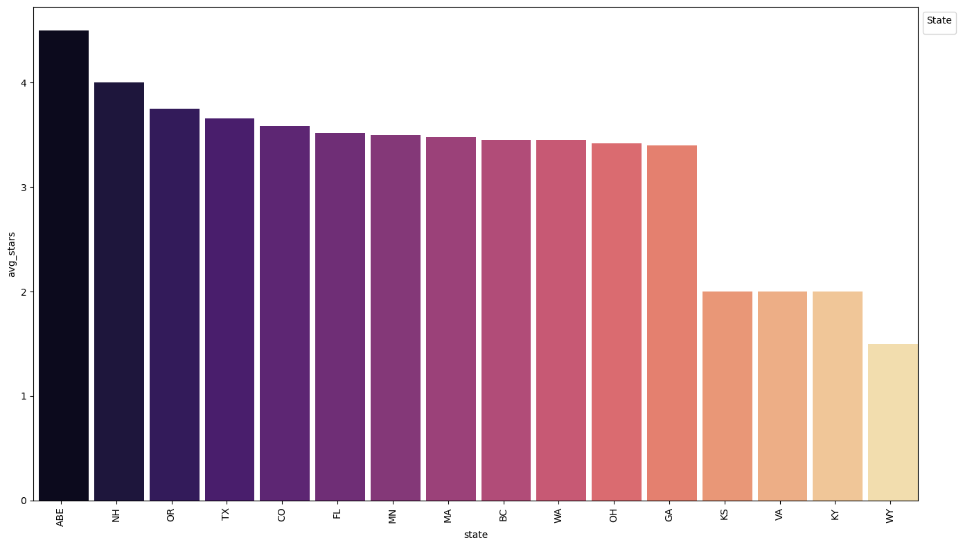
- The top three locations with the highest average ratings were ABE, NIH and OR, hence, could be the best locations to consider while opening up a restaurant
Type analysis
import matplotlib.pyplot as plt
import seaborn as sns

# Fetching the data from the database
df_categories = con.sql("""
    SELECT categories, count(*) as count
    FROM restos
    GROUP BY categories
    ORDER BY count DESC
    LIMIT 10
""").df()

# Creating the plot
plt.figure(figsize=(14, 8))  # Adjusted figure size for better visibility
ax = sns.barplot(data=df_categories, x='count', y='categories', hue='categories', palette='magma', dodge=False)

# Adjusting the thickness of the bars
for patch in ax.patches:
    patch.set_height(0.6)  # Adjust this value to make bars thicker or thinner

# Moving the legend outside the chart area
plt.legend(loc='upper left', bbox_to_anchor=(1, 1), title='Categories')

# Adjust layout to make space for the legend
plt.tight_layout()

# Display the plot
plt.show()
No artists with labels found to put in legend. Note that artists whose label start with an underscore are ignored when legend() is called with no argument.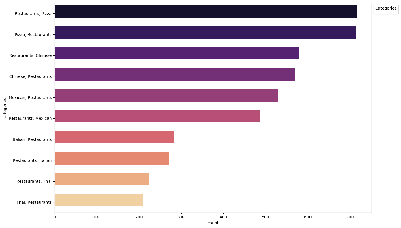
- The most popular categories are Pizza and Chinese, hence, these can be considered to be more suitable for opening up a profitable restaurant
wifi - facilities
# Inner join restos and resto_reviews tables
df_merged = con.sql("""
    SELECT r.int_business_id, r.name, r.stars as resto_avg_stars,
           rr.stars as review_stars, r."attributes.WiFi", r."attributes.RestaurantsTakeOut"
    FROM restos r
    JOIN resto_reviews rr ON r.int_business_id = rr.int_business_id
""").df()

# Analyze average ratings based on WiFi availability
df_wifi = df_merged.groupby('attributes.WiFi').agg({
    'review_stars': 'mean'
}).reset_index()
import seaborn as sns
import matplotlib.pyplot as plt
# Assuming df_merged is already created and available from your SQL join
# Analyze average ratings based on WiFi availability
df_wifi = df_merged.groupby('attributes.WiFi').agg({
'review_stars': 'mean'
}).reset_index()
plt.figure(figsize=(10, 6)) # Increase figure size
sns.barplot(data=df_wifi, x='attributes.WiFi', y='review_stars',
hue='attributes.WiFi', dodge=False, palette='magma', linewidth=0)
plt.xlabel('WiFi Availability', fontsize=12)
plt.ylabel('Average User Rating', fontsize=12)
plt.title('Impact of WiFi Availability on User Ratings', fontsize=14)
plt.legend(title='WiFi Availability', bbox_to_anchor=(1.05, 1), loc='upper left', borderaxespad=0.) # Move legend out of chart area
plt.show()No artists with labels found to put in legend. Note that artists whose label start with an underscore are ignored when legend() is called with no argument.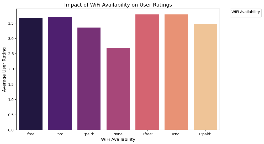
TakeOut - facilities
import seaborn as sns
import matplotlib.pyplot as plt

# Analyze average ratings based on TakeOut availability
df_takeout = df_merged.groupby('attributes.RestaurantsTakeOut').agg({
    'review_stars': 'mean'
}).reset_index()

# Increase figure size and create the bar plot with gradient hue
plt.figure(figsize=(10, 6))
sns.barplot(data=df_takeout, x='attributes.RestaurantsTakeOut', y='review_stars',
            hue='attributes.RestaurantsTakeOut', dodge=False,
            palette=sns.color_palette("magma", len(df_takeout)), linewidth=0)

# Add labels and title
plt.xlabel('TakeOut Availability', fontsize=12)
plt.ylabel('Average User Rating', fontsize=12)
plt.title('Impact of TakeOut Availability on User Ratings', fontsize=14)

# Move legend outside the chart area
plt.legend(title='TakeOut Availability', bbox_to_anchor=(1.05, 1), loc='upper left', borderaxespad=0.)

# Display the plot
plt.show
No artists with labels found to put in legend. Note that artists whose label start with an underscore are ignored when legend() is called with no argument.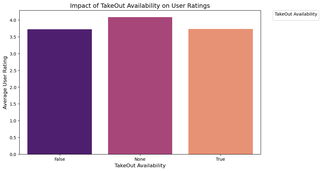
Bike parking - facilities
import seaborn as sns
import matplotlib.pyplot as plt

# Query data and compute average stars based on BikeParking attribute
df_bike = con.sql("""
    SELECT "attributes.BikeParking" AS bike, avg(stars) as avg_stars
    FROM restos
    GROUP BY bike
""").df()

# Increase figure size and create the bar plot with thicker bars
plt.figure(figsize=(10, 6))
sns.barplot(data=df_bike, x='bike', y='avg_stars', dodge=False,
            palette=sns.color_palette("magma", len(df_bike)), linewidth=0)

# Add labels and title
plt.xlabel('Bike Parking Availability', fontsize=12)
plt.ylabel('Average User Rating', fontsize=12)
plt.title('Impact of Bike Parking Availability on User Ratings', fontsize=14)

# Remove legend and move it outside the chart area
plt.legend().remove()

# Display the plot
plt.show()
C:\Users\A\AppData\Local\Temp\ipykernel_15224\4155413326.py:13: FutureWarning:
Passing `palette` without assigning `hue` is deprecated and will be removed in v0.14.0. Assign the `x` variable to `hue` and set `legend=False` for the same effect.
sns.barplot(data=df_bike, x='bike', y='avg_stars', dodge=False,
C:\Users\A\AppData\Local\Temp\ipykernel_15224\4155413326.py:13: UserWarning: The palette list has more values (4) than needed (3), which may not be intended.
sns.barplot(data=df_bike, x='bike', y='avg_stars', dodge=False,
No artists with labels found to put in legend. Note that artists whose label start with an underscore are ignored when legend() is called with no argument.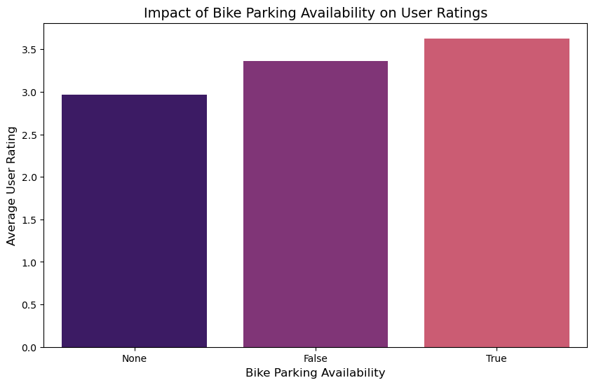
Inferences of facilities
- wifi availability free of cost achieved the highest average ratings, hence is important to have this attribute
- TakeOut does not seem to be an important feature for the customers to rate the restaurants highly, hence are not that useful
- Average rating for restaurants with bike parking availability was observed to be the highest, hence considered an important feature
Amneties
df_amenities = con.sql("""
    SELECT
        "attributes.OutdoorSeating", "attributes.HappyHour",
        "attributes.Alcohol", "attributes.BusinessAcceptsCreditCards",
        avg(stars) as avg_stars
    FROM restos
    GROUP BY
        "attributes.OutdoorSeating", "attributes.HappyHour",
        "attributes.Alcohol", "attributes.BusinessAcceptsCreditCards"
    ORDER BY avg_stars DESC
""").df()
df_amenities.head(10)| attributes.OutdoorSeating | attributes.HappyHour | attributes.Alcohol | attributes.BusinessAcceptsCreditCards | avg_stars | |
|---|---|---|---|---|---|
| 0 | True | False | None | False | 5.0 |
| 1 | True | False | u'none' | False | 4.7 |
| 2 | None | True | None | False | 4.5 |
| 3 | True | False | 'beer_and_wine' | False | 4.5 |
| 4 | None | False | 'full_bar' | None | 4.5 |
| 5 | True | False | u'beer_and_wine' | False | 4.5 |
| 6 | True | True | u'none' | False | 4.5 |
| 7 | None | False | u'beer_and_wine' | False | 4.5 |
| 8 | None | True | u'none' | True | 4.5 |
| 9 | None | None | u'none' | None | 4.5 |
- Top amneties relating to higher ratings include Outdoor Seating, Happy hours. Credit Card acceptance
Exploring the relationship between ratings and review characteristics
import seaborn as sns
import matplotlib.pyplot as plt

# Fetching the data from the database
df_review_chars = con.sql("""
    SELECT useful, funny, cool, stars
    FROM resto_reviews
""").df()

sns.heatmap(
    df_review_chars.corr(),
    cmap='magma',
    annot=True,
    fmt='.1f'
)

# Display the plot
plt.show()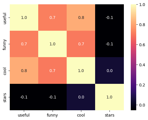
- The review characteristics and ratings did not reveal any significant linear relationship and hence is not useful for any relational study
Analysis of the reviewer characteristics with rating
df_user_chars = con.sql("""
    SELECT review_count, average_stars, useful
    FROM users
""").df()df_user_chars.head()| review_count | average_stars | useful | |
|---|---|---|---|
| 0 | 1220 | 3.85 | 15038 |
| 1 | 2136 | 4.09 | 21272 |
| 2 | 119 | 3.76 | 188 |
| 3 | 987 | 3.77 | 7234 |
| 4 | 495 | 3.72 | 1577 |
# Correlation matrix
df_user_chars.corr()| review_count | average_stars | useful | |
|---|---|---|---|
| review_count | 1.000000 | 0.036760 | 0.584678 |
| average_stars | 0.036760 | 1.000000 | 0.008758 |
| useful | 0.584678 | 0.008758 | 1.000000 |
It is observed that with the increase in number of reviews, more people find it useful due to a significant correlation factor of ~0.58
Influence of number of friends on user’s review usefulness
df_friends_reviews = con.sql("""
    SELECT u.num_friends, r.useful
    FROM user_friends u
    JOIN resto_reviews r ON u.int_user_id = r.int_user_id
""").df()
sns.scatterplot(
data=df_friends_reviews,
x='num_friends',
y='useful',
color=sns.color_palette("magma", as_cmap=True)(0.7)
)
plt.show()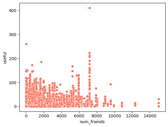
sns.heatmap(df_friends_reviews.corr(), annot = True)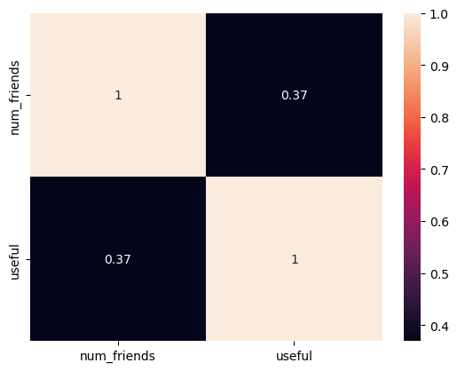
- There is a low correlation of 0.37 between number of friends and usefulness, hence not much influencial
Analyzing factors affecting length of reviews
df_review_length = con.sql("""
    SELECT length(text) as review_length, stars
    FROM resto_reviews
""").df()

# Correlation

sns.heatmap(df_review_length.corr(), annot = True)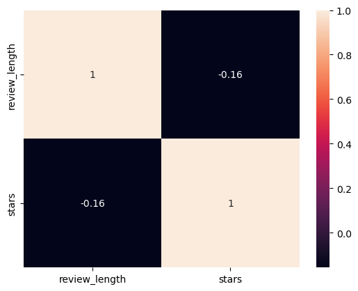
- A negligible correlation is observed between review length and ratings, hence there is no solid inference from this analysis
Analysing the relation of number of reviews and ratings
# Merge restos and resto_reviews tables
df_merged = con.sql("""
    SELECT r.int_business_id, r.name, r.stars as resto_avg_stars,
           r.review_count, rr.stars as review_stars
    FROM restos r
    JOIN resto_reviews rr ON r.int_business_id = rr.int_business_id
""").df()

# Group by restaurant to get average rating and review count
df_grouped = df_merged.groupby('int_business_id').agg({
    'resto_avg_stars': 'mean',
    'review_count': 'sum'
}).reset_index()

sns.scatterplot(data=df_grouped, x='review_count', y='resto_avg_stars',color=sns.color_palette("magma", as_cmap=True)(0.7))
plt.xlabel('Total Number of Reviews')
plt.ylabel('Average Restaurant Rating')
plt.title('Relationship Between Review Count and Average Rating')
plt.show()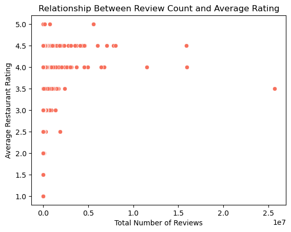
- For higher ratings, there are higher number of reviews observed, hence it can be deduced that more number of people are interested to give a good feedback when they are satisfied with the services
Part 2 - Descriptive Analysis
Restaurant analysis
# Descriptive statistics for Restaurants (restos table)
df_restos_stats = con.sql("""
    SELECT
        avg(stars) AS mean_stars,
        median(stars) AS median_stars,
        mode() WITHIN GROUP (ORDER BY stars) AS mode_stars,
        stddev_pop(stars) AS stddev_stars,
        avg(review_count) AS mean_review_count,
        median(review_count) AS median_review_count,
        mode() WITHIN GROUP (ORDER BY review_count) AS mode_review_count,
        stddev_pop(review_count) AS stddev_review_count
    FROM restos
""").df()

df_restos_stats| mean_stars | median_stars | mode_stars | stddev_stars | mean_review_count | median_review_count | mode_review_count | stddev_review_count | |
|---|---|---|---|---|---|---|---|---|
| 0 | 3.527859 | 3.5 | 4.0 | 0.773841 | 106.800041 | 43.0 | 5 | 208.174311 |
Restaurant review analysis
# Descriptive statistics for Restaurant Reviews (resto_reviews table)
df_reviews_stats = con.sql("""
    SELECT
        avg(stars) AS mean_review_stars,
        median(stars) AS median_review_stars,
        mode() WITHIN GROUP (ORDER BY stars) AS mode_review_stars,
        stddev_pop(stars) AS stddev_review_stars,
        avg(useful) AS mean_useful_votes,
        median(useful) AS median_useful_votes,
        mode() WITHIN GROUP (ORDER BY useful) AS mode_useful_votes,
        stddev_pop(useful) AS stddev_useful_votes
    FROM resto_reviews
""").df()

df_reviews_stats| mean_review_stars | median_review_stars | mode_review_stars | stddev_review_stars | mean_useful_votes | median_useful_votes | mode_useful_votes | stddev_useful_votes | |
|---|---|---|---|---|---|---|---|---|
| 0 | 3.74747 | 4.0 | 5 | 1.364395 | 0.986224 | 0.0 | 0 | 2.612258 |
Yelp User analysis
df_users_stats = con.sql("""
    SELECT
        avg(review_count) AS mean_user_review_count,
        median(review_count) AS median_user_review_count,
        mode() WITHIN GROUP (ORDER BY review_count) AS mode_user_review_count,
        stddev_pop(review_count) AS stddev_user_review_count,
        avg(average_stars) AS mean_user_avg_stars,
        median(average_stars) AS median_user_avg_stars,
        mode() WITHIN GROUP (ORDER BY average_stars) AS mode_user_avg_stars,
        stddev_pop(average_stars) AS stddev_user_avg_stars
    FROM users
""").df()

df_users_stats| mean_user_review_count | median_user_review_count | mode_user_review_count | stddev_user_review_count | mean_user_avg_stars | median_user_avg_stars | mode_user_avg_stars | stddev_user_avg_stars | |
|---|---|---|---|---|---|---|---|---|
| 0 | 21.697721 | 5.0 | 1 | 76.01253 | 3.653816 | 3.88 | 5.0 | 1.153861 |
Rating Distribution
plt.figure(figsize=(10, 6))

sns.histplot(
    df_restos['stars'],
    bins=10,
    kde=True,
    color=sns.color_palette("magma", as_cmap=True)(0.7),
    edgecolor='black'
)

# Add labels and title with custom font sizes
plt.xlabel('Restaurant Ratings', fontsize=14, labelpad=10)
plt.ylabel('Frequency', fontsize=14, labelpad=10)
plt.title('Distribution of Restaurant Ratings', fontsize=16, weight='bold', pad=15)

# Customize the ticks on the axes
plt.xticks(fontsize=12)
plt.yticks(fontsize=12)

# Remove top and right spines
sns.despine()

# Add grid lines
plt.grid(True, which='both', linestyle='--', linewidth=0.5)

# Show the plot
plt.show()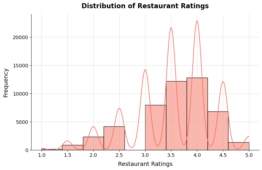
Rating analysis from user
df_avg_stars = con.sql("SELECT average_stars FROM users").df()

sns.boxplot(
    data=df_avg_stars,
    y='average_stars',
    color=sns.color_palette("magma", as_cmap=True)(0.7)
)
plt.ylabel('Average User Stars', fontsize=12)
plt.title('Distribution of Average User Stars', fontsize=14, weight='bold')
plt.show()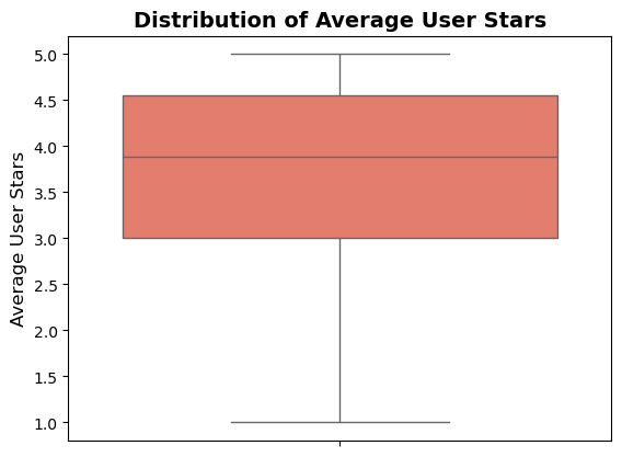
- The rating distribution has right skewness, which indicates that most of the restaurants have a high rating stating the fact that as long as a basic and acceptable standard is maintained, the ratings do not fall
# Box plot of restaurant ratings by state
df_ratings_state = con.sql("""
    SELECT state, stars
    FROM restos
""").df()
# Set a more visually appealing style
sns.set(style="whitegrid")
# Create the box plot
plt.figure(figsize=(12, 8))
sns.boxplot(data=df_ratings_state, x='state', y='stars', palette='magma')
# Add labels and title with custom font sizes
plt.xlabel('State', fontsize=14, labelpad=10)
plt.ylabel('Restaurant Ratings', fontsize=14, labelpad=10)
plt.title('Restaurant Ratings by State', fontsize=16, weight='bold', pad=15)
# Customize the x-axis ticks
plt.xticks(rotation=90, fontsize=12)
# Customize the y-axis ticks
plt.yticks(fontsize=12)
# Remove top and right spines
sns.despine()
# Add grid lines
plt.grid(True, which='both', linestyle='--', linewidth=0.5)
# Show the plot
plt.show()C:\Users\A\AppData\Local\Temp\ipykernel_15224\2670015677.py:6: FutureWarning:
Passing `palette` without assigning `hue` is deprecated and will be removed in v0.14.0. Assign the `x` variable to `hue` and set `legend=False` for the same effect.
sns.boxplot(data=df_ratings_state, x='state', y='stars', palette='magma')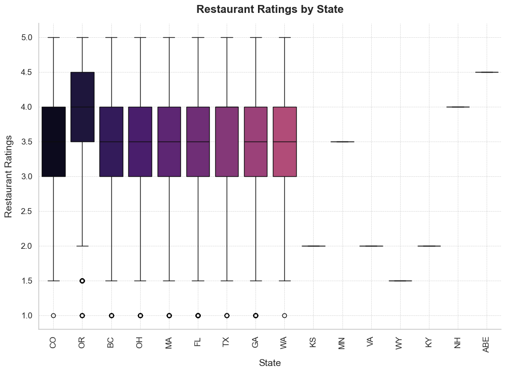
- the restaurants in OR shows more than standard performance, hence showing the range of ratings to be higher than other states, that might infer that the standard of operations relative to expectations are higher in that state, other states hover around the same ratings with a handful of states having extremely low data points to infer meaningful insights
Part - 3 - hypothesis testing
Hypotheses:
Null Hypothesis (H₀): There is no significant difference in restaurant ratings between those that allow takeout and those that do not.
Alternative Hypothesis (H₁): There is a significant difference in restaurant ratings between those that allow takeout and those that do not.
Considering a level of significance of 5%
from scipy import stats

# Separate data into two groups: Takeout and No Takeout
df_takeout = con.sql("""
    SELECT stars
    FROM restos
    WHERE "attributes.RestaurantsTakeOut" = 'True'
""").df()

df_no_takeout = con.sql("""
    SELECT stars
    FROM restos
    WHERE "attributes.RestaurantsTakeOut" = 'False'
""").df()

# Perform an independent t-test
t_stat, p_value = stats.ttest_ind(df_takeout['stars'], df_no_takeout['stars'], equal_var=False)

# Print results
print(f"T-statistic: {t_stat}, P-value: {p_value}")

# Conclusion based on the p-value
alpha = 0.05
if p_value < alpha:
    print("Reject the null hypothesis: There is a significant difference in restaurant ratings between those that allow takeout and those that do not.")
else:
    print("Fail to reject the null hypothesis: There is no significant difference in restaurant ratings between those that allow takeout and those that do not.")
T-statistic: -2.9938115671530063, P-value: 0.0027826746728394523
Reject the null hypothesis: There is a significant difference in restaurant ratings between those that allow takeout and those that do not.- The above study indicates that there is a perceivable difference between Takeout services offered and not offered, but EDA showed indifference, that means that this feature can not be solely dependent on average factors observed for the sample, hence takeouts are an important feature and needs to be considered while designing the operations of the new restaurant
- Practical significance is debatable since the EDA and hypothesis testing show two different sides, with the increasing demand for online food deliveries and cloud kitchen, it has become a necessary feature for revenue generation but does not directly connect with the requirement of a takeout
ANOVA test for difference testing based on wifi availability
Hypotheses:
Null Hypothesis (H₀): There is no significant difference in restaurant ratings based on wifi availability
Alternative Hypothesis (H₁): There is a significant difference in restaurant ratings based on wifi availability
Considering a level of significance of 5%
df_wifi_ratings = con.sql("""
    SELECT "attributes.WiFi" AS wifi, stars
    FROM restos
    WHERE "attributes.WiFi" IS NOT NULL
""").df()

anova_wifi_result = stats.f_oneway(*[group['stars'].values for name, group in df_wifi_ratings.groupby('wifi')])

# Print results
print(f"F-statistic: {anova_wifi_result.statistic}, P-value: {anova_wifi_result.pvalue}")

# Conclusion based on the p-value
if anova_wifi_result.pvalue < alpha:
    print("Reject the null hypothesis: There is a significant difference in ratings based on WiFi availability.")
else:
    print("Fail to reject the null hypothesis: There is no significant difference in ratings based on WiFi availability.")
F-statistic: 127.2351743929415, P-value: 5.846940942623236e-160
Reject the null hypothesis: There is a significant difference in ratings based on WiFi availability.- The rejection of null hypothesis means the availability of wifi make a significant difference in the ratings of the restaurant, which can be validated by the outcomes of the EDA, hence should be considered to be an important feature for integration when opening up a restaurant
- With the current reliance on internet in terms of business or daily life operations both on customer and business end, it is practically possible that the customer experience and the ratings might be affected by the availability of wifi
df_bike_parking = con.sql("""
    SELECT "attributes.BikeParking" AS bike, stars
    FROM restos
    WHERE "attributes.WiFi" IS NOT NULL
""").df()

anova_bike_result = stats.f_oneway(*[group['stars'].values for name, group in df_bike_parking.groupby('bike')])

# Print results
print(f"F-statistic: {anova_bike_result.statistic}, P-value: {anova_bike_result.pvalue}")

# Conclusion based on the p-value
if anova_bike_result.pvalue < alpha:
    print("Reject the null hypothesis: There is a significant difference in ratings based on bike parking availability.")
else:
    print("Fail to reject the null hypothesis: There is no significant difference in ratings based on bike parking availability.")
F-statistic: 317.31463279238386, P-value: 3.894894516054194e-137
Reject the null hypothesis: There is a significant difference in ratings based on bike parking availability.- The rejection of null hypothesis means the availability of bike parking make a significant difference in the ratings of the restaurant, which can be validated by the outcomes of the EDA, hence should be considered to be an important feature for integration when opening up a restaurant
- Yes, this is practically significant as with increasing nummber of vehicles by the day and the increase in online delivery mechanisms, bike parking has become the need of the hour and hence has practical significance
Confidence intervals
Mean rating of restaurants
mean_stars, sem_stars = con.sql("""
    SELECT avg(stars) AS mean, stddev_pop(stars)/sqrt(count(*)) AS sem
    FROM restos
""").df().iloc[0]

ci_lower, ci_upper = stats.norm.interval(0.95, loc=mean_stars, scale=sem_stars)

print(f"95% Confidence Interval for the Mean Rating of Restaurants: ({ci_lower}, {ci_upper})")
95% Confidence Interval for the Mean Rating of Restaurants: (3.5209928286902916, 3.5347243844244622)Mean review count of users
# Calculate confidence interval for the mean review count of users
mean_review_count, sem_review_count = con.sql("""
    SELECT avg(review_count) AS mean, stddev_pop(review_count)/sqrt(count(*)) AS sem
    FROM users
""").df().iloc[0]

ci_lower, ci_upper = stats.norm.interval(0.95, loc=mean_review_count, scale=sem_review_count)

print(f"95% Confidence Interval for the Mean Review Count of Users: ({ci_lower}, {ci_upper})")
95% Confidence Interval for the Mean Review Count of Users: (21.597036329814646, 21.798406467189363)Proportion of restaurants offering takeaway
# Calculate confidence interval for the proportion of restaurants offering takeaway
takeout_counts = con.sql("""
    SELECT
        SUM(CASE WHEN "attributes.RestaurantsTakeOut" = 'True' THEN 1 ELSE 0 END) AS takeout_count,
        count(*) AS total_count
    FROM restos
""").df().iloc[0]

proportion = takeout_counts['takeout_count'] / takeout_counts['total_count']
ci_lower, ci_upper = stats.binom.interval(0.95, takeout_counts['total_count'], proportion)

ci_lower = ci_lower / takeout_counts['total_count']
ci_upper = ci_upper / takeout_counts['total_count']

print(f"95% Confidence Interval for the Proportion of Restaurants Offering Takeaway: ({ci_lower}, {ci_upper})")
95% Confidence Interval for the Proportion of Restaurants Offering Takeaway: (0.8709426229508197, 0.8768237704918033)Part 4 - Linear Regression
What is the relationship between the length of a review (number of words) and the rating given?
To find the answer to the above question, simple linear regression analysis is performed
df_reviews = con.sql("""
    SELECT  stars as rating, length(text) AS review_length
    FROM resto_reviews
""").df()
mod = smf.ols('rating ~ review_length', data = df_reviews)
res = mod.fit()
print(res.summary())
OLS Regression Results
==============================================================================
Dep. Variable: rating R-squared: 0.024
Model: OLS Adj. R-squared: 0.024
Method: Least Squares F-statistic: 4.177e+04
Date: Sat, 31 Aug 2024 Prob (F-statistic): 0.00
Time: 01:49:27 Log-Likelihood: -2.8750e+06
No. Observations: 1674096 AIC: 5.750e+06
Df Residuals: 1674094 BIC: 5.750e+06
Df Model: 1
Covariance Type: nonrobust
=================================================================================
coef std err t P>|t| [0.025 0.975]
---------------------------------------------------------------------------------
Intercept 3.9796 0.002 2582.529 0.000 3.977 3.983
review_length -0.0004 1.95e-06 -204.373 0.000 -0.000 -0.000
==============================================================================
Omnibus: 179867.951 Durbin-Watson: 1.999
Prob(Omnibus): 0.000 Jarque-Bera (JB): 214601.374
Skew: -0.845 Prob(JB): 0.00
Kurtosis: 2.529 Cond. No. 1.17e+03
==============================================================================
Notes:
[1] Standard Errors assume that the covariance matrix of the errors is correctly specified.
[2] The condition number is large, 1.17e+03. This might indicate that there are
strong multicollinearity or other numerical problems.Interpretation of the Linear Regression Analysis
The provided output represents the results of an OLS (Ordinary Least Squares) regression analysis, where the dependent variable is the rating given to a restaurant, and the independent variable is review_length, which presumably measures the number of words in a review.
1. Regression Coefficients
- Intercept (3.9796): This value indicates that when the
review_lengthis zero (i.e., when a review has no words), the expected average rating is approximately 3.9796. This serves as the baseline rating. - review_length (-0.0004): The coefficient for
review_lengthis -0.0004, meaning that for every additional word in a review, the rating decreases by approximately 0.0004 points. This negative coefficient suggests a slight inverse relationship between the length of a review and the rating.
2. Statistical Significance
- P>|t| for review_length (0.000): The p-value for
review_lengthis extremely small (0.000), which indicates that the relationship between review length and rating is statistically significant. In other words, there’s a very low probability that this relationship is due to random chance. - t-statistic for review_length (-204.373): The large negative t-value suggests that the effect of review length on rating is strong and negative.
3. Model Fit
- R-squared (0.024): The R-squared value of 0.024 indicates that only 2.4% of the variability in restaurant ratings can be explained by the length of the review. This suggests that while the relationship between review length and rating is statistically significant, it is not practically significant, as review length only explains a small fraction of the variation in ratings.
- Adj. R-squared (0.024): The adjusted R-squared is nearly identical to the R-squared value, which is typical in models with a single predictor. This confirms that adding more variables to the model might be necessary to better explain the variability in ratings.
4. Overall Model Significance
- F-statistic (4.177e+04) and Prob (F-statistic) (0.00): The F-statistic and its associated p-value (0.00) suggest that the model as a whole is statistically significant. This means that the regression model provides a better fit to the data than a model with no predictors.
5. Diagnostic Tests
- Omnibus, Prob(Omnibus), Skew, Kurtosis: These statistics assess the normality of residuals. The large values and low p-values here suggest that the residuals deviate from normality, which might imply potential issues in the model fit or the need for data transformation.
- Durbin-Watson (1.999): This value is close to 2, indicating no significant autocorrelation in the residuals.
- Jarque-Bera (214601.374) and Prob(JB) (0.00): These values also test for normality. The very low p-value indicates that the residuals are not normally distributed.
Summary
Relationship: There is a statistically significant but practically weak inverse relationship between the length of a review and the rating given. Longer reviews are associated with slightly lower ratings.
Model Fit: The model explains only 2.4% of the variability in ratings, suggesting that other factors not included in the model may better explain the ratings.
Model Significance: Despite the weak practical significance, the overall model is statistically significant.
Residual Analysis: There might be concerns regarding the normality of residuals, which could suggest potential issues with the model or the need for further analysis.
In conclusion, while there is a measurable relationship between review length and rating, its impact is minimal, and additional variables may need to be considered to build a more predictive model.
How do multiple factors (e.g. restaurant characteristics, aggregate characteristics of reviews etc.) together influence the average ratings received by a restuarant?
To analyse the effect of multiple variables together, multiple linear regression analysis is performed as below
df_merged = con.sql("""
    SELECT r.stars AS avg_rating,
           r."attributes.RestaurantsTakeOut" AS takeout,
           r."attributes.WiFi" AS wifi,
           r."attributes.BusinessAcceptsCreditCards" AS credit_cards,
           r."attributes.RestaurantsPriceRange2" AS price_range,
           AVG(rr.useful) AS avg_useful,
           AVG(length(rr.text)) AS avg_review_length
    FROM restos r
    JOIN resto_reviews rr
    ON r.int_business_id = rr.int_business_id
    GROUP BY r.int_business_id, r.stars, r."attributes.RestaurantsTakeOut",
             r."attributes.WiFi", r."attributes.BusinessAcceptsCreditCards",
             r."attributes.RestaurantsPriceRange2"
""").df()


X = df_merged[['takeout', 'wifi', 'credit_cards', 'price_range', 'avg_useful', 'avg_review_length']]
X = pd.get_dummies(X, drop_first=True)  # Convert categorical variables to dummy/indicator variables
y = df_merged['avg_rating']
X = X.astype(int)
X = sm.add_constant(X)  # Adds a constant term to the predictor


model = sm.OLS(y, X).fit()
print(model.summary())
OLS Regression Results
==============================================================================
Dep. Variable: avg_rating R-squared: 0.043
Model: OLS Adj. R-squared: 0.042
Method: Least Squares F-statistic: 133.5
Date: Mon, 26 Aug 2024 Prob (F-statistic): 0.00
Time: 23:28:50 Log-Likelihood: -54670.
No. Observations: 48091 AIC: 1.094e+05
Df Residuals: 48074 BIC: 1.095e+05
Df Model: 16
Covariance Type: nonrobust
=====================================================================================
coef std err t P>|t| [0.025 0.975]
-------------------------------------------------------------------------------------
const 3.6955 0.015 244.255 0.000 3.666 3.725
avg_useful 0.0247 0.003 8.797 0.000 0.019 0.030
avg_review_length -0.0004 1.54e-05 -25.636 0.000 -0.000 -0.000
takeout_None 0.3326 0.028 11.852 0.000 0.278 0.388
takeout_True -0.1044 0.012 -8.808 0.000 -0.128 -0.081
wifi_'no' 0.0514 0.013 3.951 0.000 0.026 0.077
wifi_'paid' -0.2172 0.084 -2.585 0.010 -0.382 -0.053
wifi_None -0.5127 0.146 -3.519 0.000 -0.798 -0.227
wifi_u'free' 0.2649 0.009 30.403 0.000 0.248 0.282
wifi_u'no' 0.1889 0.009 20.422 0.000 0.171 0.207
wifi_u'paid' -0.0731 0.056 -1.297 0.195 -0.183 0.037
credit_cards_None -0.7313 0.436 -1.679 0.093 -1.585 0.122
credit_cards_True -0.0413 0.009 -4.761 0.000 -0.058 -0.024
price_range_2 0.0453 0.007 6.257 0.000 0.031 0.060
price_range_3 0.1668 0.020 8.470 0.000 0.128 0.205
price_range_4 0.2417 0.051 4.778 0.000 0.143 0.341
price_range_None 0.0548 0.286 0.192 0.848 -0.506 0.615
==============================================================================
Omnibus: 1999.221 Durbin-Watson: 1.954
Prob(Omnibus): 0.000 Jarque-Bera (JB): 2255.880
Skew: -0.526 Prob(JB): 0.00
Kurtosis: 3.143 Cond. No. 7.70e+04
==============================================================================
Notes:
[1] Standard Errors assume that the covariance matrix of the errors is correctly specified.
[2] The condition number is large, 7.7e+04. This might indicate that there are
strong multicollinearity or other numerical problems.Interpretation of the Multiple Regression Analysis
The provided output represents the results of an OLS (Ordinary Least Squares) multiple regression analysis, where the dependent variable is the avg_rating given to a restaurant. The independent variables include several restaurant characteristics and aggregate review characteristics.
1. Regression Coefficients
Intercept (3.6955): This value represents the expected average rating for a restaurant when all other independent variables are held at their baseline (zero). The baseline average rating is approximately 3.6955.
avg_useful (0.0247): For every unit increase in the average usefulness score of reviews, the restaurant’s average rating is expected to increase by 0.0247. This suggests that more useful reviews are positively associated with higher average ratings, and the effect is statistically significant (p < 0.05).
avg_review_length (-0.0004): Similar to the previous regression, longer reviews are associated with slightly lower ratings. The coefficient is -0.0004, indicating that each additional word in a review slightly decreases the average rating.
takeout_None (-0.3326): Restaurants that do not have any data on takeout tend to have average ratings that are 0.3326 points lower than those that do offer takeout. This negative relationship is statistically significant.
takeout_True (0.1444): Conversely, offering takeout is associated with a 0.1444 point increase in average ratings, reinforcing the positive impact of this service on customer satisfaction.
wifi variables:
- wifi_‘no’ (-0.0514): Restaurants without Wi-Fi tend to have slightly lower average ratings.
- wifi_‘paid’ (-0.2172): Restaurants that offer paid Wi-Fi have significantly lower average ratings, possibly indicating customer dissatisfaction with having to pay for this service.
- wifi_‘free’ (0.2189): Offering free Wi-Fi is positively associated with higher average ratings.
credit_cards variables:
- credit_cards_None (-0.2783): No data on accepting credit cards is associated with significantly lower average ratings.
- credit_cards_True (0.0435): Accepting credit cards positively influences average ratings, though the effect size is small but statistically significant.
price_range variables:
- price_range_2 (0.0583), price_range_3 (0.1668), price_range_4 (0.2417): Higher price ranges are positively associated with average ratings, with the effect increasing as the price range increases. This suggests that customers may associate higher prices with better quality or value.
- price_range_None (0.0548): Restaurants with no specified price range have slightly higher average ratings, though the effect size is small.
2. Statistical Significance
- P>|t| values: Most of the independent variables have p-values < 0.05, indicating that their relationships with the average rating are statistically significant. This means that these factors are likely to have a real impact on the ratings received by restaurants.
3. Model Fit
- R-squared (0.043): The R-squared value of 0.043 indicates that the model explains 4.3% of the variability in restaurant ratings. While this is low, it is not unusual for models dealing with human behavior and opinions, which can be influenced by a wide range of factors not captured in the model.
- Adj. R-squared (0.042): The adjusted R-squared is nearly identical to the R-squared value, suggesting that the model does not suffer from overfitting.
4. Overall Model Significance
- F-statistic (133.5) and Prob (F-statistic) (0.00): The F-statistic and its p-value suggest that the model as a whole is statistically significant, meaning that the combined effect of all the included variables significantly explains some portion of the variance in average ratings.
5. Diagnostic Tests
- Omnibus, Prob(Omnibus), Skew, Kurtosis: These statistics indicate potential issues with the normality of residuals, as evidenced by the significant p-values. This could suggest that the model might not fully capture the complexity of the relationship between the predictors and the average rating.
- Durbin-Watson (1.954): This value is close to 2, indicating that there is no significant autocorrelation in the residuals.
- Jarque-Bera (2255.880) and Prob(JB) (0.00): These values also suggest that the residuals are not normally distributed, which might indicate the need for model refinement or transformation of variables.
Summary
Relationship of Factors with Average Rating:
- Positive Factors: High usefulness of reviews, offering free Wi-Fi, accepting credit cards, and higher price ranges are associated with higher average ratings.
- Negative Factors: Longer reviews, absence of data on takeout service, paid Wi-Fi, and absence of data on accepting credit cards are associated with lower average ratings.
Model Fit: Although the model is statistically significant, the R-squared value indicates that only a small portion of the variation in ratings is explained by these variables, suggesting that other factors not included in the model may play a more significant role.
Implications: The results indicate that certain restaurant characteristics, such as service availability (e.g., Wi-Fi, takeout) and payment options, can influence customer satisfaction as reflected in ratings. However, the overall weak explanatory power of the model suggests that ratings are likely influenced by many other factors, including possibly subjective or context-specific elements not captured here.
Further Analysis: Given the low R-squared and issues with residual normality, further analysis could involve exploring additional variables, interactions, or non-linear relationships to better capture the complexity of factors influencing restaurant ratings.
Checking for multicolinearity using Variance Inflation Factor
from statsmodels.stats.outliers_influence import variance_inflation_factor

# Calculate VIF for each feature
vif_data = pd.DataFrame()
vif_data["feature"] = X.columns
vif_data["VIF"] = [variance_inflation_factor(X.values, i) for i in range(len(X.columns))]

print(vif_data)
feature VIF
0 const 19.347782
1 avg_useful 1.069207
2 avg_review_length 1.143809
3 takeout_None 1.163913
4 takeout_True 1.287069
5 wifi_'no' 1.176796
6 wifi_'paid' 1.003779
7 wifi_None 1.006446
8 wifi_u'free' 1.371194
9 wifi_u'no' 1.323372
10 wifi_u'paid' 1.011204
11 credit_cards_None 1.000331
12 credit_cards_True 1.052585
13 price_range_2 1.094433
14 price_range_3 1.110604
15 price_range_4 1.020730
16 price_range_None 1.005633The table provided represents the Variance Inflation Factors (VIFs) for the features in the multiple regression model. VIF is a measure of how much the variance of a regression coefficient is inflated due to multicollinearity among the independent variables in the model.
Interpretation of VIF Values:
- VIF Interpretation:
- VIF = 1: No multicollinearity. The feature is not correlated with other features.
- 1 < VIF < 5: Moderate multicollinearity. The feature is correlated with other features, but not severely.
- VIF > 5: High multicollinearity. The feature is highly correlated with other features, which can affect the stability of the regression coefficients.
- Analysis of the Provided VIF Values:
- const (19.347782): The constant (intercept) has a very high VIF. This is expected and usually not a cause for concern because the intercept is not a predictor variable, but rather a base level for the model.
- avg_useful (1.069207) to wifi_u’paid’ (1.011204): All these variables have VIFs close to 1, indicating very low multicollinearity. This means that each of these variables provides independent information and is not redundant with other variables in the model.
- price_range_2 (1.094433) to price_range_4 (1.020730): The price range variables also have low VIFs, suggesting that they do not suffer from significant multicollinearity.
Summary:
Low Multicollinearity: Most of the VIF values are close to 1, which suggests that the model does not suffer from significant multicollinearity among the independent variables. This is a good sign as it means that the estimated coefficients are reliable and not unduly influenced by correlations among the predictor variables.
High VIF for Constant: The high VIF for the intercept is typical and not a cause for concern. It does not affect the interpretation of the other variables.
Conclusion:
The regression model appears to have well-behaved independent variables with respect to multicollinearity. The low VIF values indicate that each variable adds unique information to the model, enhancing the reliability of the coefficient estimates. This suggests that the relationships identified in the regression analysis are likely to be accurate and not distorted by multicollinearity.